

On this article, I’ll clarify the differential equations of fluid movement, i.e., conservation of mass (the continuity equation. So with out losing any time, allow us to begin.
What’s differential Evaluation?
As part of this text, it’s important to know what differential evaluation is and the way we will apply it to elucidate continuity and Naiver Stroke’s theorem.
A few of the important key factors associated to the differential evaluation are as follows:
Differential evaluation is the appliance of a differential equation of fluid movement to any or each level within the circulation subject over a area referred to as the Circulation Area.
Some readers may confuse the phrase differential with the small management volumes piled up on one another within the circulation subject.
At any time when the scale of the management quantity crosses the restrict and extends to infinity, then the scale of every management quantity turns into so small that the conservation equations simplify to a set of partial differential equations. These partial equations can simply be relevant every time required in any circulation subject.
As I’ve mentioned earlier, two differential equations, the Regulation of Conservation of Mass (Continuity Equation) and Newton’s Second Regulation (Naiver Strokes Equation), are those on which there’s a drastic change within the temperature and density such form of equations are simply solved with the assistance of differential equation.
The next diagram reveals the research of management quantity during which the management quantity appears to be a lot much like the black field.
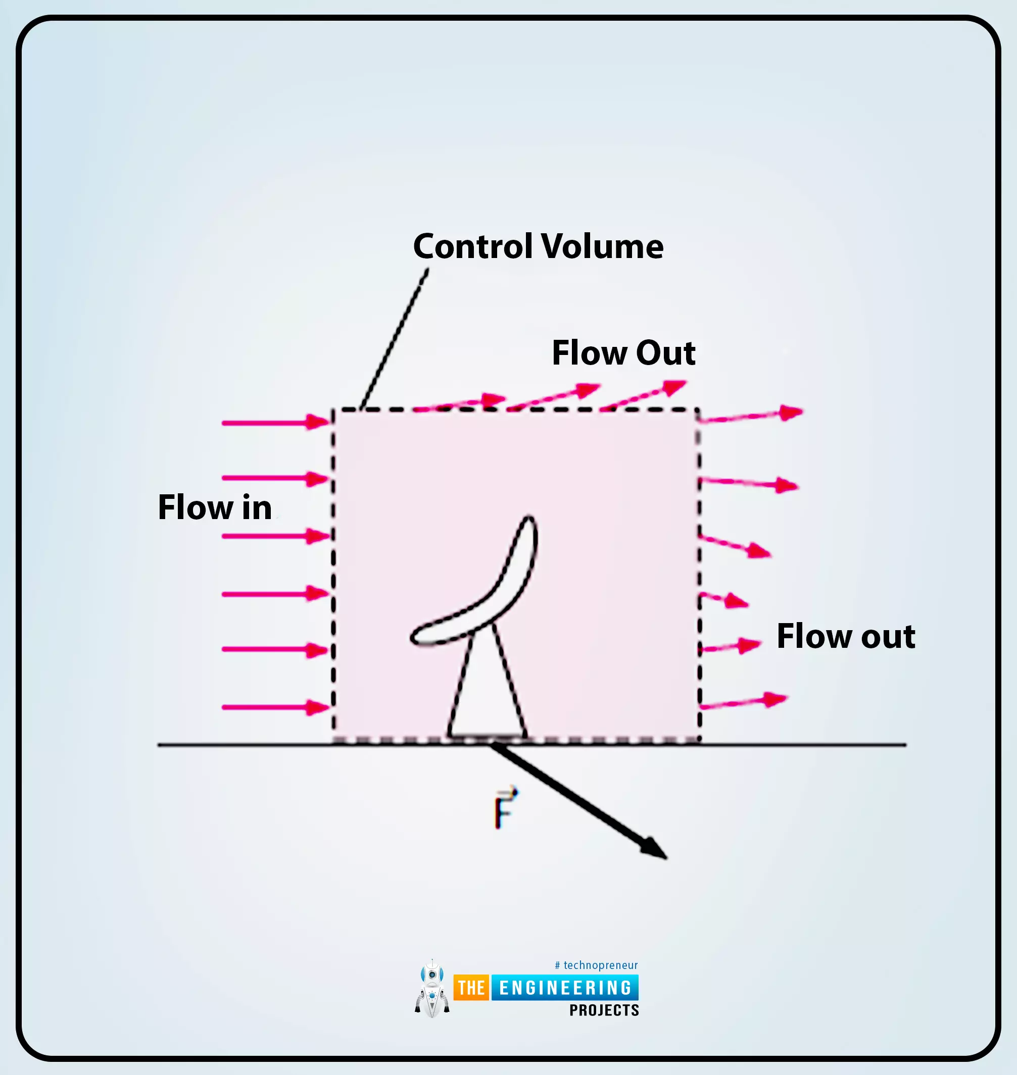

Whereas fixing the differential equation within the case of incompressible circulation, there are about 4 unknown, i.e., velocity parts (u, v, w), one stress element, and 4 equations (three equations from Naiver Strokes Regulation and one from Regulation of Conservation of Mass).
There are variables and constants in equations, however in differential equations, all of the variables are solved without delay as a result of, in such conditions, the equations are coupled. Now, what’s coupled, and the way are equations coupled? We’ll see it within the upcoming subjects.
Whereas fixing the differential equation, the boundary circumstances should be outlined.
We’re transferring in direction of the primary vital a part of our article, i.e., the Regulation of Conservation of Mass. Allow us to begin.
Conservation of Mass–Continuity Equation
In certainly one of my earlier articles, I’ve extensively defined the conservation of mass. However now, right here, I’ll clarify the derivation by way of the infinitesimal management quantity by the divergence theorem. So let’s begin.
To elucidate the subject, I’ll divide it into important essential factors within the following method.
0=∫CV∂ρ∂t dV+∫CSV.n dA (a)
The equation is for the mounted and management volumes.
∫CV∂ρ∂tdV=inm-outn (b)
Now I’ll clarify the derivation utilizing the divergence theorem.
Derivation Utilizing the Divergence Theorem:
The opposite title of the divergence theorem known as Gauss’s Theorem.
The assertion of the divergence theorem is as follows:
The Divergence Theorem (Gauss’s Theorem) is used to rework a quantity integral of the divergence of a vector into an space integral over the floor that defines the amount.
A few of the important key factors associated to the Divergence theorem are as follows:
∫vV.GdV=∮AG.n dA (c)
There are two sorts of integration within the equation one is easy, and the opposite has circled it. This means that your entire space surrounds the amount. In order you’ll be able to see that the equation is useful in gaining information.
The first goal of utilizing the divergence theorem is to rework the amount integral of the divergence vector into an space integral over the floor, and that floor defines the amount.
Within the case of any vector, the divergence can be outlined as a G, and the equation as m can be used to explain it.
In some circumstances, we additionally outline the divergence as follows:
G=ρV
We will additionally outline it by taking part in with the values, and for that, we substitute the worth of equation (c) into equation (a), and we’ll get the outcomes as follows:
0=∫cv∂ρ∂t dV+∫cvV. (ρV) dV
As you’ll be able to see that there are two integrals, so to get the required equation, we’ll mix the 2 integrals into one after which the consequence can be as follows:
∫cv∂ρ∂t+V. VdV=0
Now, we come to the conclusion that the equation that’s talked about above is for the management volumes, no matter any dimension and form.
So, the assertion above is barely doable if the phrases inside the brackets are identically zero.
Transferring in direction of the essential assertion, i.e. the equation of continuity. So the final differential equation for the conservation of mass is often known as the continuity equation, and the equation is as follows:
∂ρ∂t+V. V=0
So, that is the equation of continuity. This equation is for compressible flows solely and doesn’t implement for incompressible ones; the -mentioned equation ensures the validity of the circulation area level.
Now that’s all from the derivation utilizing the divergence theorem. The subsequent matter can also be part of it. Take a look.
Derivation utilizing an Infinitesimal Management Quantity
The continuity theorem is outlined in numerous methods, and certainly one of them will describe by me. The continuity theorem begins with the management quantity, and, taking it as a base, I’ll inform the entire matter.
So following are some important key factors associated to the subject:
We’ll begin with the belief. Allow us to contemplate an infinitesimal field that controls quantity and aligns with the axes within the Cartesian Coordinates system.
The next is the diagram that reveals the box-shaped management quantity.
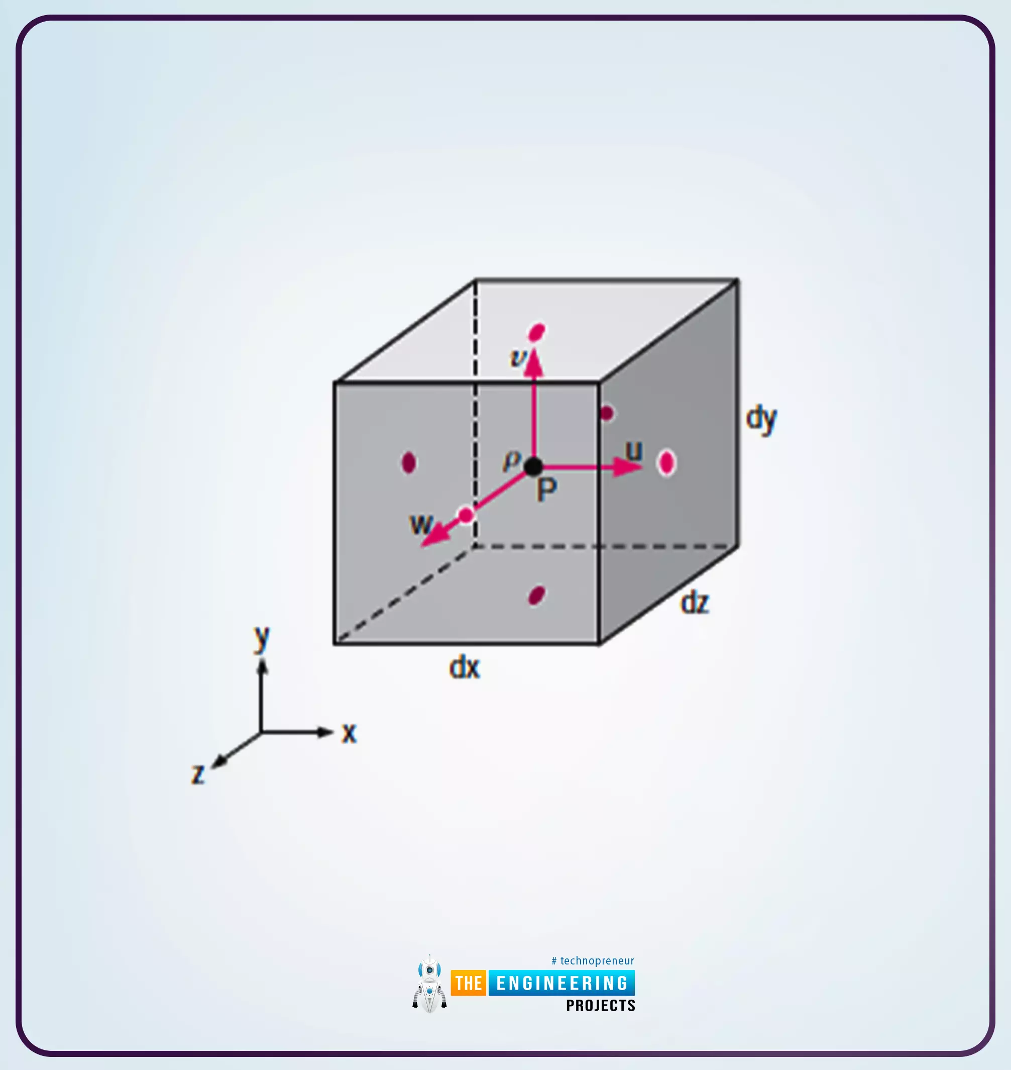
As you’ll be able to see from the diagram alongside the x-direction, the size is talked about as dx, within the y-direction as dy and alongside the z-direction because the dz, respectively.
Furthermore, on the centre of the field, there may be info that claims that the density is outlined as an emblem and the rate is outlined in velocity parts as u, v, and w, respectively.
So, we use Taylor’s Theorem inside the field at completely different places away from the centre. And to outline this level, we’ll use an instance as follows:
(u)centre of proper face=ρu+∂(ρu)∂xdx2+12!2(ρu)x2(dx2)2
Within the case of the above-mentioned equation, the management quantity has simply restricted to some extent solely, and the upper energy and even the second energy phrases are negligible.
So, for the six faces of the field, we use the Taylor collection enlargement to density instances the traditional velocity element on the central level of every of the six faces, so they’re as follows:
(u)centre of proper face≅ ρu+∂(ρu)∂xdx2
(u)centre of left face≅ ρu-∂(ρu)∂xdx2
(w)centre of entrance face≅ ρw+∂(ρw)∂zdz2
(w)centre of rear face≅ ρw-∂(ρw)∂zdz2
(v)centre of prime face≅ ρv+∂(ρv)∂ydy2
(v)centre of backside face≅ ρv-∂(ρv)∂ydy2
The mass circulation price into or out of the faces of the field is the same as the density instances the traditional velocity parts on the centre level of the face instances the floor space of the face.
m=VnA
The above equation is legitimate for every face. The Vn reveals the magnitude of the traditional velocity by the face, and the A reveals the floor areas of the face.
The next diagram reveals the mass circulation price by every face of our infinitesimal management quantity; you’ll simply get the concept about it:
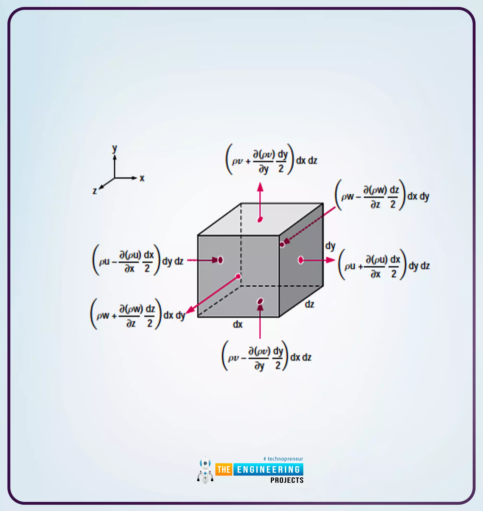
So all of the theoretical background that I’ve talked about within the diagram that’s above might be simply comprehensible by the diagram.
For all of the nonnormal velocity parts, the truncated Taylor collection expansions on the centre of every face may also be outlined. However we’ve not represented as these parts are tangential to the face.
Now we’ll transfer in direction of one other equation, and that equation says the management quantity shrinks at any of some extent, and the worth of the amount integral on the left aspect of the equation (b) will develop into as follows:
∫cv∂ρ∂t dV≅∂ρ∂tdxdydz
As we all know that the amount of the field is dx, dy, and dz, respectively.
Here’s a trick: with the assistance of the diagram, we will apply the approximations from the determine to the correct aspect of the equation talked about above. On this case, we’ll add all of the mass circulation charges on the inlet and the outlet of the management quantity by the entire faces. Then take a left, backside, and again faces contributing to the mass circulation price. Then in regards to the equation, the correct aspect can be as follows:
inm≅(ρu-ρu∂xdx2)dydz+ρv-ρv∂ydy2dxdz+(ρw-ρw∂zdz2)dxdy
The next are the faces which are talked about within the equation:
Left Face =ρu-ρu∂xdx2dydz
Backside Face=ρv-ρv∂ydy2
Rear Face=(ρw-ρw∂zdz2)dxdy
The subsequent matter can also be a part of the Continuity Equation. So with out losing any time, allow us to begin.
Different Type of the Continuity Equation
There’s additionally an alternate option to current the continuity equation as we all know that the next equation is in keeping with the product rule of divergence theorem:
∂ρ∂t+V. V=∂ρ∂t+V. ρ+ρ.V=0
In an effort to clarify the continuity equation various method, I’ll clarify it in a couple of vital key factors:
1DρDt+.V=0
The above-mentioned equations present the fluid ingredient that’s flowing by the circulation subject, and additionally it is referred to as the fabric ingredient. Right here there’s a change that the .V is the change within the density.
So we will say that if the change within the density of the fabric ingredient (fluid ingredient) is small as in comparison with the magnitudes of the rate gradient within the .V additionally if the ingredient strikes round, then the circulation is alleged to be incompressible, and it’s restricted to it solely.
So that’s all from the choice method of presenting the continuity equation. Now the following matter is one other a part of presenting the continuity equation.
Continuity Equation in Cylindrical Coordinates
The cylindrical polar coordinates system is a method of presenting the phrases in (r,,z). additionally it is often known as the cylindrical coordinates system.
On this matter, I’ll present you ways the phrases might be defined in a cylindrical system, and it’s one other method of presenting the continuity equation. So following are a number of the vital key factors associated to the subject. Take a look at it:
There might be three-dimensional, one-dimensional and two-dimensional cylindrical coordinates, however right here on this matter in the beginning, I’ll clarify by way of the two-coordinates system solely.
The next are the reason of the (r, θ):
Right here, r reveals the radial distance i.e., from the origin to any level (allow us to say P).
Then there comes , now which reveals the angular measurement from the x-axis (if we speak about usually, then is outlined as a constructive worth, and it’s in a counterclockwise route).

Within the case of three-dimensional, there may be clearly a z-axis. So with a view to present the factors, the next diagrams clarify nicely. Take a look at it.
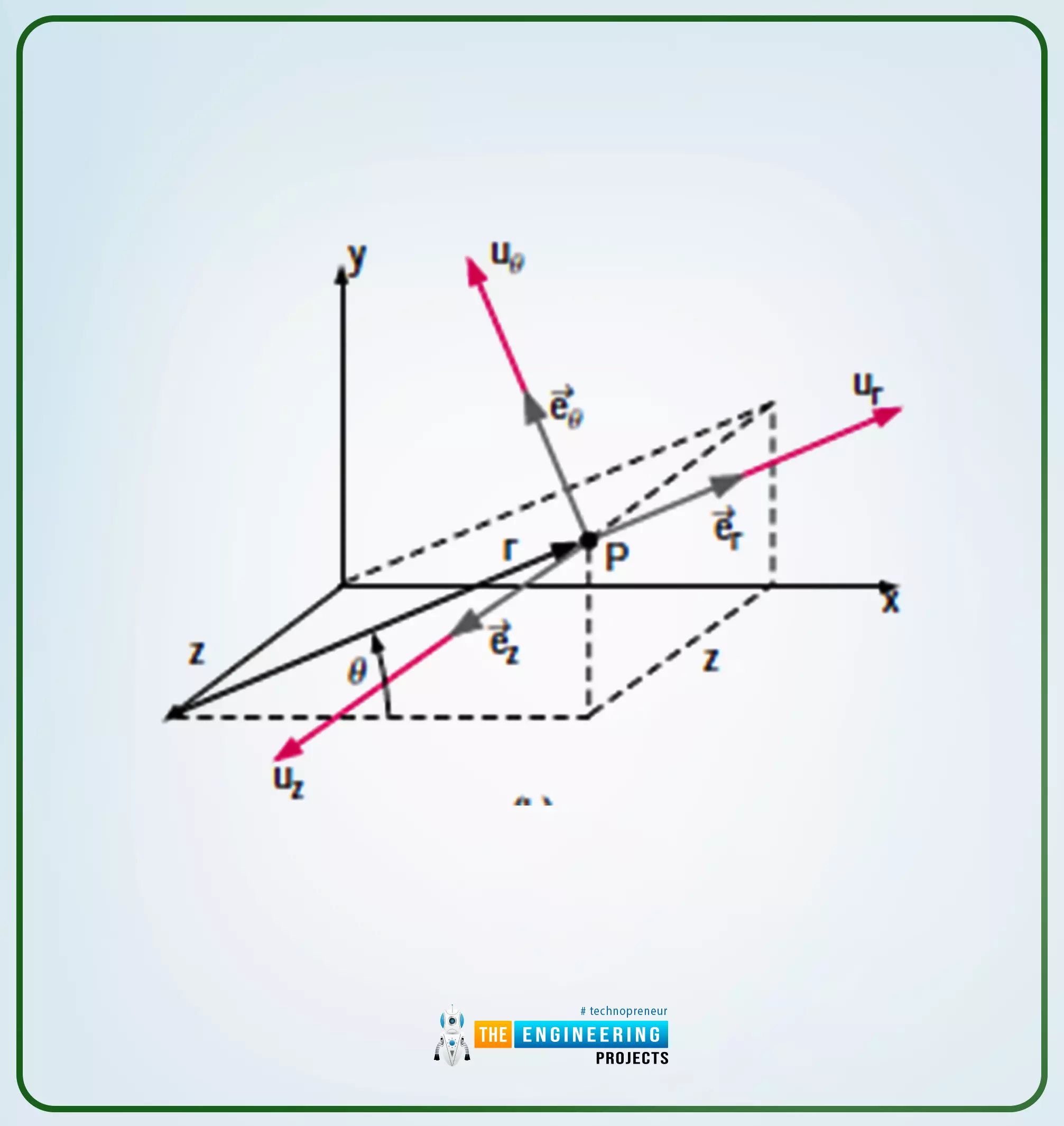
In order you’ll be able to see that within the three-dimension case, there are two extra values, one for the rate element and the second for the unit vector.
So the next equation reveals the coordinate transformation:
r=x2+y2
x=rcos
y=sin
θ=yx
∂ρ∂t+1r(rρur)r+1r(rρu)+1r(rρuz)z =0
Thanks for studying.


0 Comments